A Straightforward Guide to A/B Testing

A/B Testing can be extremely useful during experimentation. Adding statistical rigor to situations where you compare one option against another. This is one step which can help guard against making faulty conclusions.

This article will demonstrate the critical steps in an A/B test:

Determining Minimum Detectable Effect
Calculating Sample Size
Analyzing Results for Statistical Significance

Scenario Overview

To demonstrate a situation where a company may employ A/B testing, I’m going to create a fictitious video game dataset.

In this scenario, a video game development company has recognized lots of users are quit playing after one particular level. A hypothesis posed by the product team is that the level is too hard, and making it easier will allow for less user frustration and ultimately more players continuing to play the game.

Sample Size Calculation

Desired Business Effect

Our video game company has made some tweaks to the level to make it easier, effectively changing the difficulty from hard to medium. Before blindly rolling an update out to all the users, the product team wants to test the changes on a small sample to see if they make a positive impact.

The desired metric is the percentage of players who continue playing after reaching our level in question. Currently, 70% of users continue to play where the remaining 30% stop playing. The product team has decided increasing this to 75% would warrant deploying the changes and making an update to the game.

Minimum Detectable Effect

This piece of information (70% to 75%) helps us calculate the minimum detectable effect - one of the inputs to calculating sample size. Our problem is testing two proportions, so we’ll use the proportion_effectsize function in statsmodels to translate this change into something we can work with.

import statsmodels.api as sm

init_prop = 0.7
mde_prop = 0.75
effect_size = sm.stats.proportion_effectsize(
    init_prop, 
    mde_prop
)
print(f'For a change from {init_prop:.2f} to {mde_prop:.2f} - the effect size is {effect_size:.2f}.')

Output: For a change from 0.70 to 0.75 - the effect size is -0.11.

Sample Size

Now that we have our minimum detectable effect, we can calculate sample size. To do this for a proportion problem, zt ind solve power is used (also from the statsmodels library).

We set the nobs1 (number of observations of sample 1) parameter to None which signifies this is what we are looking to solve for.

A significance level of 0.05 and power of 0.8 are commonly chosen default values, but these can be adjusted based on the scenario and desired false positive vs. false negative sensitivity.

from math import ceil

sample_size = sm.stats.zt_ind_solve_power(
    effect_size=effect_size, 
    nobs1=None, 
    alpha=0.05, 
    power=0.8
)
print(f'{ceil(sample_size)} sample size required given power analysis and input parameters.')

Output: 1250 sample size required given power analysis and input parameters.

Experiment Data Overview

After communicating the sample size needed to the product team, an experiment was run where a random sample of 1,250 players played the new easier level and another 1,250 played the hard level.

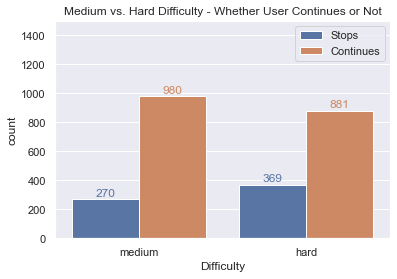
After gathering the data, we learn that 980 users (of 1,250) continued playing after reaching the medium difficulty level while 881 (of 1,250) continued playing after reaching the hard difficulty level. This seems decent enough and above our hope of at least 5% improvement, should we make the change?

Before deciding, it’s important to test for statistical significance to guard against the possibility that this difference could have occurred simply by random chance (accounting for our significance and power).

Analyzing Results

Calculating Inputs

The statistical test we’ll use is the proportions_ztest. We need to calculate a number of inputs first - the number of successes and observations. Data is stored in a pandas dataframe with columns for medium and hard - with 0 representing users that stopped playing and 1 representing those that continued.

# Get z test requirements
medium_successes = df.loc[:, 'medium'].sum()
hard_successes = df.loc[:, 'hard'].sum()
medium_trials = df.loc[:, 'medium'].count()
hard_trials = df.loc[:, 'hard'].count()

print(f'Medium: {medium_successes} successes of {medium_trials} trials. Hard: {hard_successes} successes of {hard_trials} trials.')

Output: Medium: 980 successes of 1250 trials. Hard: 881 successes of 1250 trials.

Performing the Z Test

Performing the z test is simple with the required inputs:

from statsmodels.stats.proportion import proportions_ztest

# Perform z test
z_stat, p_value = proportions_ztest(
    count=[medium_successes, hard_successes], 
    nobs=[medium_trials, hard_trials]
)
print(f'z stat of {z_stat:.3f} and p value of {p_value:.4f}.')

Output: z stat of 4.539 and p value of 0.0000.

A p value below 0.05 meets our criteria. Reducing the level difficulty to medium is the way to go!

Summary

While this is a fictitious and straightforward example, utilizing a similar approach in the real world can add some rigor to your experiments. Consider using A/B testing when you have two samples you are looking to gauge whether an experiment resulted in a significant change or not based on your desired metric.

All examples and files available on Github.