Speed up Linear Regression with Matrix Math

Linear Regression is an extremely popular and useful model. It’s used by Excel Gurus and Data Scientists alike - but how can we fit lots of regression models quickly? This article walks through various ways to fit a linear regression model and how to speed things up with some Linear Algebra.

In this article, I’ll walk through a few different approaches for ordinary least squares linear regression.

1. Fitting a model using the statsmodels library
2. Fitting a Simple Linear Regression using just Numpy
3. Using the Matrix Formulation
4. How to fit multiple models with one pass over grouped data
5. Comparing performance of looping vs. matrix approaches

Data Overview

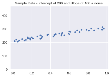
The data utilized in this article will be generated sample data. Using numpy + introducing some random noise, the below dataset has been created to use for demonstrating OLS fitting techniques. This data will be stored in X and y variables for the next few examples.

Statsmodels OLS

One great approach for fitting a linear model is utilizing the statsmodels library. We simply pass in our two variables, call the fit method, and can retrieve results via a call to summary(). Note - these parameters can also be accessed directly using fit.params.

import statsmodels.api as sm

fit = sm.OLS(y, X).fit()
fit.summary()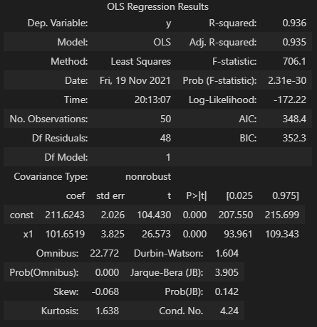

The above results show a number of details, but for this walkthrough we’ll focus on the coefficients. You’ll see under the ceof column, the y intercept (labeled const) is ~211.62 and our one x regressor coefficient is 101.65. This fits in well with expectations given the parameters and randomness introduced to the initial dataset.

Numpy Arithmetic Solution for Simple Linear Regression

If we are dealing with just one regressor/independent variable (similar to this example), then it is pretty straightforward to solve for the slope and intercept directly.

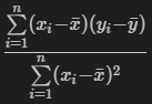
Looking at the above formula, it’s the summation of x less it’s mean times y less it’s mean, divided by the x calculation squared. The intercept can also be found using this slope and the means of x and y as a second step.

This coefficient formula is straightforward to carry out directly in numpy with a couple lines of code. The dot function in numpy will take care of our sumproducts and we can call .mean() directly on the vectors to find the respective averages.

Finally, we check that the results of our numpy solution exactly match the statsmodels version using the allclose function.

import numpy as np

x = X[:,1] # reduce extra intercept dimension
slope = np.dot(x - x.mean(), y - y.mean()) / np.dot(x - x.mean(), x - x.mean())
print(f'Simple linear regression arithmetic slope of {slope:.2f} vs. statsmodels ols fit slope of {fit.params[1]:.2f}.')
print(f'Results equal: {np.allclose(slope,fit.params[1])}')

Simple linear regression arithmetic slope of 101.65 vs. statsmodels ols fit slope of 101.65.
Results equal: True

Matrix Formula

The matrix formula extends OLS linear regression one step further - allowing us to derive the intercept and slope from X and y directly, even for multiple regressors. This formula is as follows, for a detailed derivation check out this writeup from economic theory blog.

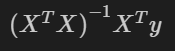
The numpy code below mirrors the formula quite directly. You could also use dot products here, but matmul is used as this fits our next scenario better when extending to three dimensions (multiple models fitted at once).

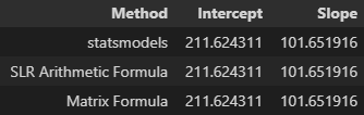
matrix_intercept, matrix_slope = np.matmul(np.matmul(np.linalg.inv(np.matmul(X.T,X)), X.T), y)

Before moving on to the next step with new datasets, a quick check of each method reveals the same intercept and slope - three different ways of achieving the same thing for the use case of simple linear regression.

Multiple Regressions at Once

Use Case Examples

Moving on to our next use case, what if you want to run multiple regressions at once? Let’s say you have a retail dataset with various stores, and you wanted to run ols regressions independently on each store - perhaps to compare coefficients or for finer grained linear model fits.

Another example use case - an ecommerce store may want to run a number of ols linear regressions over monthly sales data by product. They want to fit linear models independently in order to get a rough sense of directionality and trend over time by observing various models’ coefficients.

Data Shape and Multiple Matrix Formula

To demonstrate, a dataset with 2 sets of 50 data points is created. Both have 2 regressors/independent variables, but we want to fit a linear model of each of the two groupings separately.

The data has a shape of (2, 50, 3) - representing 2 groupings, 50 data points in each, and 2 independent variables for each (+ intercept). Our Y variable is now (2, 50) - 2 groupings, 50 data points.

If we try to plug this into our statsmodels ols function, we’ll get an error. However, we can extend our matrix formula to find the intercepts/slopes for each model in one pass. Let’s define mathematically what we are trying to accomplish:

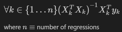
For n regressions (2 in this case) with each individual regression grouping of data represented by k, we want to run the matrix version of ols linear regression we performed in the previous section. You’ll see this is the same formula as the prior section, we are just introducing performing multiple iterations (k = 1 to n), one set of matrix multiplications for each grouping.

Numpy Transpose Adjustments

Implementing this in numpy requires a few simple changes. If we just plugged our X and y variables directly into the prior formulation, the dimensions wouldn’t line up how we want. The reason this happens is using the same transpose function (.T in numpy) will change our shape from (2, 50, 3) to (3, 50, 2). Not exactly what we want…

The numpy matmul documentation specifies if more than 2 dimensions is passed in with either argument, the operation is treated as a stack of matrices residing in the last two indexes. This is the behavior we are looking for, so the first dimension should remain as 2 (stacking our groupings) and we just want to transpose the 50 and 3.

We can use the transpose function and specify how to transpose our axes exactly to get the right shape. Passing in axes (0,2,1) will get the desired shape - swapping the last to axes, but keeping our n regressions dimension in place to stack over.

For the following code examples, X will now be referred to as X_many and similarly for y in order to differentiate from prior examples.

X_many.transpose(0,2,1).shape

(2, 3, 50)

Revised Numpy Operations

With this transpose knowledge in mind, time to make the changes to solve this grouped version. For readability, the numpy code has been split into two lines. Transpose is modified to work along the proper dimensions and an additional empty axis is added to y_many just to line up the matmul operation.

x_operations = np.matmul(np.linalg.inv(np.matmul(X_many.transpose(0,2,1),X_many)), X_many.transpose(0,2,1))
m_solve = np.matmul(x_operations, y_many[..., np.newaxis])[...,0]
m_solve

array([[209.9240413375,  95.3254823487,  61.4157238175],
       [514.164936664 ,   8.1355322839,   4.3353162671]])

We get back an array that contains our intercept and coefficient for each independent variable. Performing a similar (but looped) operation using statsmodels and using numpy.allclose to check reveals that the coefficients are the same.

We were able to fit many regressions at once. This approach can be helpful in cases where we want to fit a bunch of linear models that are grouped and partitioned by one particular dimension and solved independently.

Einsum Notation

We can also solve this with the einsum function in numpy. This uses Einstein summation convention to specify how operations are performed. At a high level, we define the subscripts for each matrix as a string - if the order is swapped that specifies a transpose and multiplication occurs over common letters. For more information, check out the numpy docs as they walk through a few examples.

The einsum version has been broken out into a few more steps for readability. Inside the notation string, we are specifying the transposes along with the matrix multiplication to be performed. This also allows us to handle the np.newaxis piece of code by instead specifying the output dimensions.

# Step 1: inv of XXt
step1 = np.linalg.inv(np.einsum('ikj,ikl->ijl', X_many, X_many))
# Step 2: Above operation matmul Xt
step2 = np.einsum('ijk,ilk->ijl', step1, X_many)
# Step 3: Above operation matmul y
einsum_solve = np.einsum('ijk,ik->ij', step2, y_many)
# Print Results
print(einsum_solve)

[[209.9240413375  95.3254823487  61.4157238175]
 [514.164936664    8.1355322839   4.3353162671]]

This gives us the same results as prior version, although performance can be a tad slower. If you are familiar with einsum notation, this can be a useful implementation.

Speed Comparison

Groupby/Apply Pattern

One way I’ve seen multiple regressions implemented at once is using a pandas dataframe with the groupby/apply method. In this method, we define a function and pandas will split the dataset into groupings and apply that function - returning and reducing the results as needed.

This is the use case in our “grouped regression”. Switching our numpy arrays into one dataframe, grouping by a regression_number column, and applying a custom ols function that fits and returns the results will provide for the same coefficients (although pandas displays with a bit few decimal points).

# For each regression we are attempting to do in parallel, run the run_sm_ols function
df.groupby('regression_number').apply(run_sm_ols)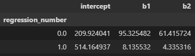

Comparing Performance

Now that we have two different ways of performing OLS over multiple groupings, how do they perform?

For this test, instead of 2 groupings of 50 points and 2 regressors, we’ll expand to 100 groupings and 3 regressors - shape of (100, 50, 4) - as a more realistic scenario.

Running a timeit test in our notebook using the %%timeit magic command shows the pandas groupby/apply approach takes 120 milliseconds while the numpy matrix version takes only 0.151 milliseconds. Matrix Multiplication was almost 800 times faster!

Granted, I’m sure there are ways to optimize the pandas implementation, but the nice part about the matrix version is a few lines of code directly in numpy is already fast.

Summary

Understanding the math behind certain basic approaches to machine learning can allow you to customize and extend approaches where needed. Many open source libraries are fast, well tested, and often do exactly what you need them to.

However, there may be one-off situations where implementing a simple, but well-understood approach such as linear regression using numpy can yield better performance without too much additional complexity.

All examples and files available on Github.