How To Forecast in Python Using Arima

Overview

Part 1 Recap

A prior article in this series reviewed how to use seasonal decomposition to parse out seasonal and trend components. In this article, the trend and residual components of our seasonal decomposition will be used to make a time series forecasting model. Then, seasonal components will be added back to see how the full forecast looks compared to actuals.

Review Part 1: How To Find Seasonality Using Python, which covered these steps:

1. Overview of the data: We’ll be forecasting Kansas City Crime data - more specifically the number of Breaking & Entering crimes per month.
2. Loading Data: Data was loaded in using Pandas and then normalized to get the number of crimes per day for each month.
3. Seasonal Decomposition: The seasonal decompose function from the Python statsmodels library helped break out the data into trend and seasonal components.

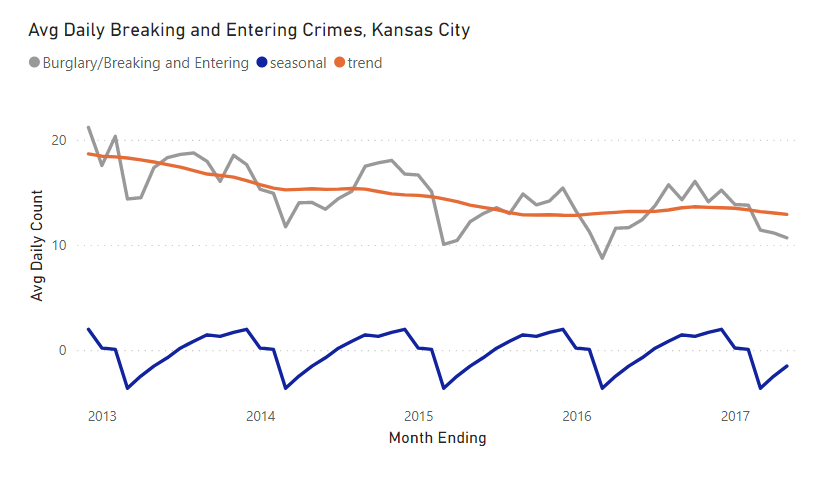
Starting Dataset

In this article, the we pick up using the seasonally decomposed data. This looks as follows:

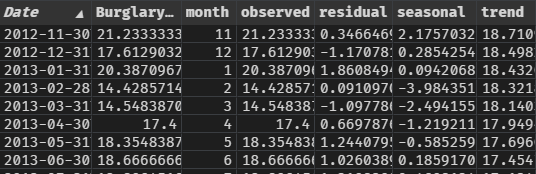
• Date: Month end date from source data.
• Burglary: Normalized count metric from source data.
• Month: Parsing out the month from date.
• Observed: Matches Burglary column (added via seasonal decompose).
• Residual: Amount not explained by seasonal or trend.
• Seasonal: Seasonal component of decomposition.
• Trend: Trend component of decomposition.

The idea here will be to use a sum of residual and trend components and feed that into our ARIMA model to forecast into the future. Then we’ll simply add back seasonality piece to get to a forecast that is comparable with our source data.

Modeling

Train Test Split

From the original dataset, the time series is split up into two components - df_train and df_test - in order to separate training and testing. Seasonal decompose was re-run on the training set only, giving a similar dataset to the previous image, but excluding the most recent 12 months.

# Train/Test Split
df_train = df[:-12].copy()
df_test = df[-12:].copy()

# Re-Run Seasonal Decompose (train data only) 
sd = seasonal_decompose(df_train['Burglary/Breaking and Entering'], period=12)
combine_seasonal_cols(df_train, sd) # custom helper function combining original and seasonal columns

Combining Columns

The next step is to combine our trend and residual columns, in order to feed into the ARIMA model. The thought is, trend and any additional patterns in the residual component can be captured by ARIMA and seasonality added back in after the forecast is made (since it is a constant by month).

# Trend and Residual combination
df_train['trend_plus_resid'] = df_train['trend'] + df_train['residual']
df_train = df_train[df_train.trend_plus_resid.notnull()]

Fit ARIMA

For this example, SARIMAX is used. In the event any additional variables need to be added as inputs, this function will make that possible at a later stage (the “X” in SARIMAX). Additionally, I picked the default order parameter. This can be further tuned, but left as-is/default for now.

# Sarimax
sm = SARIMAX(
    df_train.trend_plus_resid, 
    order=(1,0,0) # to be tuned/optimized in a future article
) 
res = sm.fit()

Out Of Sample Forecast

The forecast will be done using the predict method from our results object. The start and end dates are simply implied from our test dataframe. This will allow us to make an out-of-sample forecast that can be compared against the original data to see how accurate we are.

# Make trend forecast
df_test['trend_prediction'] = res.predict(
    start=np.min(df_test.index), 
    end=np.max(df_test.index)
)

Seasonal Add Back

The final step is to add back the seasonal component. The code below does the following:

1. Parse out the seasonal piece of our training results. This is the same for each year, so we just need a slice of 12 months to join to whatever prediction month we are making in our test set.
2. Combine the seasonal deltas with our predictions. The next two lines combine the seasonal piece with the predictions made from trend and residuals in the prior step. This adds together seasonality and our trend/residual based forecast to get a full forward-looking prediction.
3. Combine with original dataset for visualization. This last line is option, joining our prediction with our original data based on the date index. This helps line everything up to be visualized in one chart.

# Add Seasonal component
seasonal_prediction = df_train[-12:].reset_index()[['month', 'seasonal']]
df_test = df_test.reset_index().merge(
    seasonal_prediction, 
    how='left', 
    left_on='month', 
    right_on='month'
).set_index('Date')
df_test['combined_prediction'] = df_test['trend_prediction'] + df_test['seasonal']

# Add to orignal df for visualization
df['prediction'] = df_test['combined_prediction']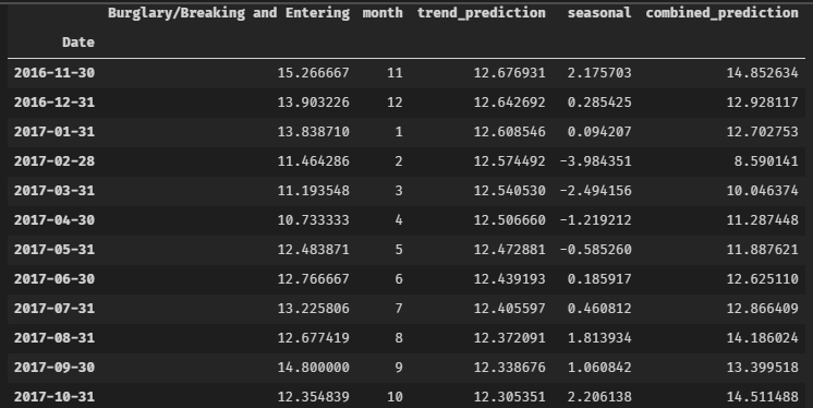

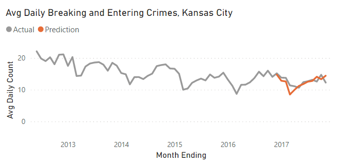
Results

The final results are as follows. We didn’t optimize or tune the SARIMAX parameters (will be covered in a future article), but as you can see the out-of-sample forecast matched the test results pretty well. Many of the errors can be seen as matching some historical trends (ex: the usually larger degree of low points in February).

Summary

Using the statsmodels library in Python, we were able forecast a seasonally decomposed dataset using ARIMA. This approach extended the trend/residual components and then added back the same seasonal ups and downs into the future.

Interested in your thoughts, if you found this approach helpful or have used different approaches in the past to solve similar issues - comment below!

All examples and files available on Github.