How To Find Seasonality Using Python

Parsing seasonality from time series data can often be useful in data analytics. It helps with analyzing seasonality for decision making as well as for more accurate forecasts. Python can be used to separate out these trend and seasonal components.

Dataset

Overview

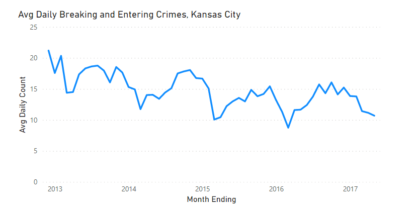
The time series data we’ll be analyzing is the Kansas City Crime Summary - more specifically the number of Breaking & Entering crimes per month. Do you think there will be any seasonal components to this data? Let’s find out.

Initial Visualization

To start, the original data is visualized below using Power BI - this helps to see any seasonality that can be spotted visually. There appears to be an overall downward trend and what looks like some seasonality as well - February is often the lowest point, while crimes increase in the summer and into the Holidays.

However, how much is related to seasonality vs. trend and how would we automate separation of seasonality components?

Seasonal Decomposition

Overview

The statsmodels library in Python has a seasonal_decompose function that does just this. Given a time series of data, the function splits into separate trend, seasonality, and residual (noise) components.

After loading and reformatting the data, the date and metric will be fed into this function to parse out the separate pieces.

Data Load

To get the data in the right shape, there are 4 main steps to take:

1. Read in the data: Data will be read into a pandas dataframe using the pandas.read_csv function.
2. Pull out just the date and metric columns: We only need the date component (monthly for this dataset) and metric (the Burglary/Breaking and Entering column).
3. Normalize the data: Since each month has a different number of days, dividing the monthly totals by number of days in the month gives a more comparable average daily count to use.
4. Set the dataframe date index: Setting our date column to be the index of the pandas dataframe allows for an easier setup when using the seasonal decompose function. Additional examples on setting an index can be found here.

The code for these four steps is as follows:

# Load Data
df = pd.read_csv("../data/Kansas_City_Crime__NIBRS__Summary.csv")

# Choose only necessary columns
df = df[['Date', 'Burglary/Breaking and Entering']]

# Normalize Metric
df['Burglary/Breaking and Entering'] = \
    df['Burglary/Breaking and Entering'] \
        / pd.to_datetime(df['Date']).dt.day

# Set date index
df = set_date_index(df, 'Date') # custom helper function

There is one custom function used as a helper, set date index, to abstract away date formatting into a separate function.

It creates a copy of the dataframe (to leave the original data intact), sets the date column to a datetime type, and finally sorts and sets the index.

def set_date_index(input_df, col_name='Date'):
    """Given a pandas df, parse and set date column to index.
        col_name will be removed and set as datetime index.

    Args:
        input_df (pandas dataframe): Original pandas dataframe
        col_name (string): Name of date column

    Returns:
        pandas dataframe: modified and sorted dataframe
    """
    # Copy df to prevent changing original
    modified_df = input_df.copy()

    # Infer datetime from col
    modified_df[col_name] = pd.to_datetime(modified_df[col_name])

    # Sort and set index
    modified_df.sort_values(col_name, inplace=True)
    modified_df.set_index(col_name, inplace=True)

    return modified_df

Trend vs. Seasonality

The next piece is actually running the seasonal decomposition. The dataframe is passed in as an argument as well as period=12 to represent our monthly data and find year-over-year seasonality.

# Seasonal decompose
sd = seasonal_decompose(df, period=12)
combine_seasonal_cols(df, sd) # custom helper function

One additional helper function was used to simply add the results to our original dataframe as new columns.

def combine_seasonal_cols(input_df, seasonal_model_results):
    """Adds inplace new seasonal cols to df given seasonal results

    Args:
        input_df (pandas dataframe)
        seasonal_model_results (statsmodels DecomposeResult object)
    """
    # Add results to original df
    input_df['observed'] = seasonal_model_results.observed
    input_df['residual'] = seasonal_model_results.resid
    input_df['seasonal'] = seasonal_model_results.seasonal
    input_df['trend'] = seasonal_model_results.trend

Output

Finally the results were written to a local csv file to be visualized in Power BI. If this was a recurring process, we could setup an API or use cloud services to host our model; however, for a one-time run a local csv file will do just fine.

df.to_csv("../data/results.csv")

Visualize Results

Visualizing the final result, the new seasonal (dark blue) and trend (orange) lines are added to the original chart.

A slight downwards trend has been identified along with a seasonal component (adding or subtracting up to 4 crimes per day from the trend).

The neat part of this methodology is that the trend, seasonal, and residual components are additive back to the original time series. You’ll see in the visualization below, adding the trend and seasonal components more or less gets back to the original dataset (residual/noise is the remaining piece).

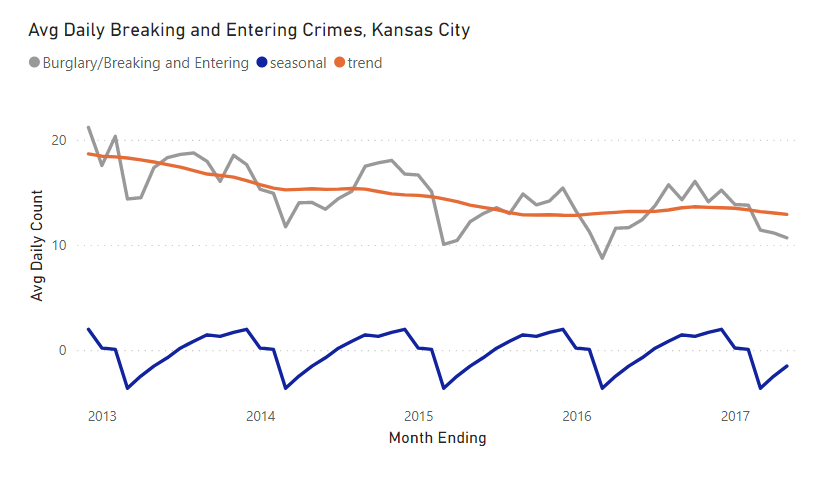
Crimes seem to be lowest in February due to seasonality (cold weather?), and ramp up throughout the summer months and into the holidays.

Summary

Using the statsmodels library in Python, we were able to separate out a time series into seasonal and trend components. This can be useful for forecasting - for example, extending a trend and then adding back the same seasonal ups and downs into the future. It can also be helpful when analyzing degree seasonality is important - ex: if you wanted to see what time of year to focus resources.

Interested in your thoughts, if you found this approach helpful or have used different approaches in the past to solve similar issues - comment below!

All examples and files available on Github.