Sliced Aggregates in Power BI

Different modeling approaches can speed up performance of your Power BI dataset - albeit with the tradeoff of additional complexity.

One situation is where users need to access a very large dataset, but typically apply the same set of filters - resulting in a small subset of rows meeting the needs of most queries. A sliced aggregate approach (implemented in the data model + DAX) can be used to make your models performant where they need to be, but still allow the full range of reporting.

Data Model

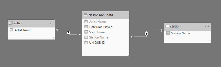
For demonstration purposes, the dataset is classic rock songs played on the radio (full dataset sourced from FiveThirtyEight). I’ve taken the data and broken out artist and station into dimensional components. The tables are as follows:

• Artist: Contains the artist name (ex: “The Black Crowes”).
• Station: Name of the station who played the song (ex: KSHE is the local St. Louis classic rock station.)
• Classic-Rock-Data: Fact table containing a row for each play of a song.

Sliced Aggregates

The main fact table has ~37k rows in total. Let’s say we’re compiling this dataset for St. Louisans, and we know (for the most part) users filter to the KSHE station. On a much lower frequency, they might look at other portions of the dataset. With this in mind, we want the KSHE “queries” to load fast - with less performance emphasis on other types of queries.

The first step is to create an aggregate table, with only the “common” slice of data included. Referencing the classic rock fact table, I used Power Query to create a new table with just KSHE as the station.

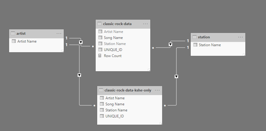
Then in DAX, I modified my Song Count measure to pull from this smaller aggregate when the conditions match (Selected Station = “KSHE”) - giving the same result with hopefully increased performance.

Metric Chooser (Song Count) = 
var sliced_agg =
IF(
    SELECTEDVALUE('station'[Station Name]) = "KSHE", 
    TRUE(),
    FALSE()
)

RETURN
IF(
    sliced_agg,
    DISTINCTCOUNT('classic-rock-data-kshe-only'[UNIQUE_ID]),
    DISTINCTCOUNT('classic-rock-data'[UNIQUE_ID])
)

Testing

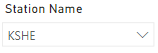
This can be tested using Dax Studio. Running a trace, we can show the engine is using the smaller sliced agg table when KSHE is the only station.

SELECT
  DCOUNT ( 'classic rock data kshe only'[UNIQUE ID] )
FROM 'classic rock data kshe only'
LEFT OUTER JOIN 'station' 
  ON 'classic rock data kshe only'[Station Name]='station'[Station Name]
WHERE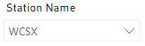
	'station'[Station Name] = 'KSHE';

Additionally, the full table is used when the selection doesn’t meet the criteria.

SELECT
  DCOUNT ( 'classic rock data'[UNIQUE ID] )
FROM 'classic rock data'
LEFT OUTER JOIN 'station' 
  ON 'classic rock data'[CALLSIGN]='station'[Station Name]
WHERE
	'station'[Station Name] = 'WCSX';

Caveats and Summary Takeaways

This was a small example - adding complexity to optimize performance by targeting ~2k row table instead of filtering a ~37k row table likely has a negligible impact. However, expanding this out to enterprise scale where the full table has millions of rows vs. the smaller table at a fraction of the size - you may see performance improvements.

One additional note to be aware of, this example does involve some data duplication. The KSHE records were included in both fact tables. Depending on the size, performance tradeoffs, mixed vs. all import model, etc - there are likely situations where this is not ideal.

Interested in your thoughts, if you find this approach helpful or have used different approaches to solve similar issues - comment below!

Note: The model and DAX are available on Github for those interested.