Building classification models on data that has largely imbalanced classes can be difficult. Using techniques such as oversampling, undersampling, resampling combinations, and custom filtering can improve accuracy.

In this article, I’ll walk through a few different approaches to deal with data imbalance in classification tasks.

1. Oversampling
2. Undersampling
3. Combining Oversampling and Undersampling
4. Custom Filtering and Sampling

Scenario and Data Overview

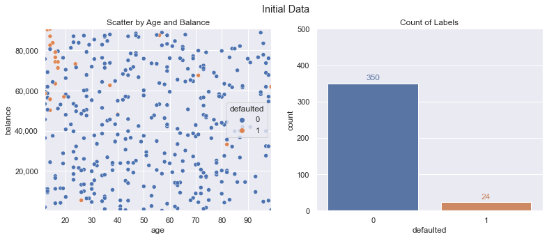
To demonstrate various class imbalance techniques, a fictitious dataset of credit card defaults will be used. In our scenario, we are trying to build an explainable classifier that takes two inputs (age and card balance) and predicts whether someone will miss an upcoming payment.

A mock up of the data is shown in the following charts. You’ll see there are some random defaults (orange dots) throughout the data, but they make up a small percentage (24 out of 374 training example instances, ~6.4%). This can make it challenging for some machine learning classification algorithms to pick up on, and we may want to limit our potential set of model choices in certain cases for explainability/regulation factors.

For this scenario, our goal will be 90%+ on accuracy and 50%+ on F1 score (harmonic mean of precision/recall) using logistic regression.

Baseline Logistic Regression

For a baseline model to use for comparisons, we’ll run a simple logistic regression and plot the decision bounds, as well as calculate various accuracy metrics.

The base logistic regression meets our 90%+ accuracy goal, but fails on the precision/recall front. You’ll see why below, with such a small relative size of the defaulted class, the model is just predicting every single data point as not defaulted (represented by the light blue background in decision boundary plot).

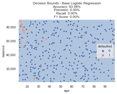
However, there is a clear section in the top left of our data (very young age with high balances) that seem to default more often than randomly. Can we do any better when incorporating resampling methods?

Oversampling

One popular method to dealing with this problem is oversampling using SMOTE. Imbalanced learn is a python library that provides many different methods for classification tasks with imbalanced classes. One of the popular oversampling methods is SMOTE.

SMOTE stands for Synthetic Minority Over-sampling Technique. Given the name, you can probably intuit what it does - creating synthetic additional data points for the class with fewer data points. It does this by taking into account other features - you can almost think of it as using interpolation between the few samples we do have to add new data points where they might exist.

Applying SMOTE is straightforward; we simply pass in our x/y training data and get back the desired resampled data. Plotting this new data, we now show an even distribution of classes (350 defaulted vs. 350 not defaulted). A lot of new defaulted class data points were created, which should allow our model to learn a function that doesn’t just predict the same outcome for every data point.

from imblearn.over_sampling import SMOTE

# Oversample using SMOTE
sm = SMOTE(random_state=42)
x_train_smote, y_train_smote = sm.fit_resample(x_train, y_train)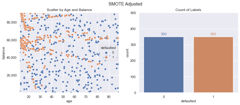

Fitting a new logistic regression model on this resampled data yields the decision boundary below.

You can see now that instead of a blue background representing a non default decision for the entire chart (as our baseline model did), this new model trained on SMOTE resampled data is predicting the top left portion defaulting (represented with a light orange background).

from sklearn.linear_model import LogisticRegression

# Logistic Regression
clf = LogisticRegression()
clf.fit(x_train_smote, y_train_smote)
predictions = clf.predict(x_train_smote)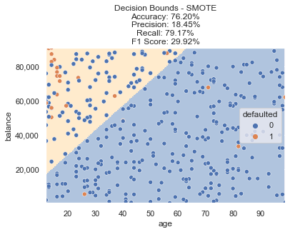

Oversampling the class that only had a few data points certainly led to a higher percentage of default predictions, but did we accomplish our goals? Accuracy dropped to ~76%, but F1 score increased to ~30%. Not quite there yet, let’s try some additional methods to see if this can be improved.

Undersampling

The opposite of oversampling the class with fewer examples is undersampling the class with more. Using the approach of Edited Nearest Neighbors we can strategically undersample data points. Doing this leads to the following modified training data - we still have our 24 default class data points, but the majority class now only has 287 of the original 350 data points in our new training dataset.

from imblearn.under_sampling import EditedNearestNeighbours

enn = EditedNearestNeighbours()
x_train_enn, y_train_enn = enn.fit_resample(x_train, y_train)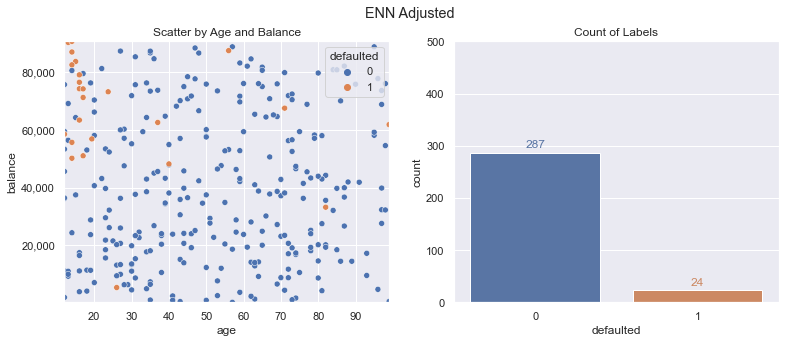

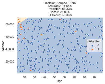
This results in the following decision bounds. The model properly targets the top left as the most frequently defaulted region, but the F1 score isn’t where we need it to be. There are certainly data points still on the table that can be captured to create a more ideal decision boundary.

Undersampling + Oversampling

Another popular method is combining the two approaches. We can oversample using SMOTE and then clean the data points using ENN. This is referred to as SMOTEENN in imblearn.

from imblearn.combine import SMOTEENN

smoteenn = SMOTEENN(random_state=42)
x_train_smoteenn, y_train_smoteenn = smoteenn.fit_resample(x_train, y_train)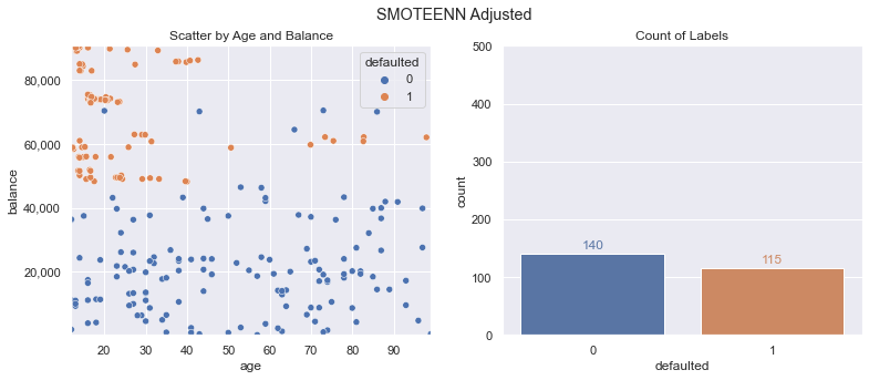

Our count of labels is a lot closer to equal, but we have fewer overall data points. How does this do on our metrics?

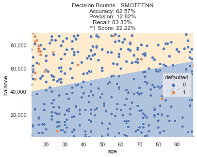
This method resulted in a bit more of an extreme decision boundary, with a further drop in accuracy and lower F1 score.

Custom Sampling + SMOTE

For our data, SMOTE seems to help, but maybe we can be a bit more targeted with which data points we want to oversample. One approach we can take is using a simple K Nearest Neighbors classifier and pick just the data points that have neighbors also belonging to our defaulted class with some probability threshold.

from sklearn.preprocessing import StandardScaler
from sklearn.neighbors import KNeighborsClassifier

# Scale Features
scaler = StandardScaler()
x_train_scaled = scaler.fit_transform(x_train)

# Fit KNN
knn = KNeighborsClassifier(n_neighbors=3)
knn.fit(x_train_scaled, y_train)
preds = pd.DataFrame(knn.predict_proba(x_train_scaled))
preds.columns = ['label_0', 'label_1']

# Bind defaulted label proba to train dataset
x_train['knn_minority_class_proba'] = preds['label_1']

# Filter X and Y Custom
x_train_filtered = x_train.loc[(x_train.knn_minority_class_proba > 0.5) | (y_train == 0), :]
y_train_filtered = y_train.loc[(x_train.knn_minority_class_proba > 0.5) | (y_train == 0)]

With this in place, we now have the following set of data - reducing our defaulted class from 24 to 10 (but hopefully getting rid of the noisy data points that may be throwing off our SMOTE processes and creating too aggressive interpolations).

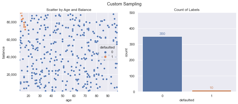
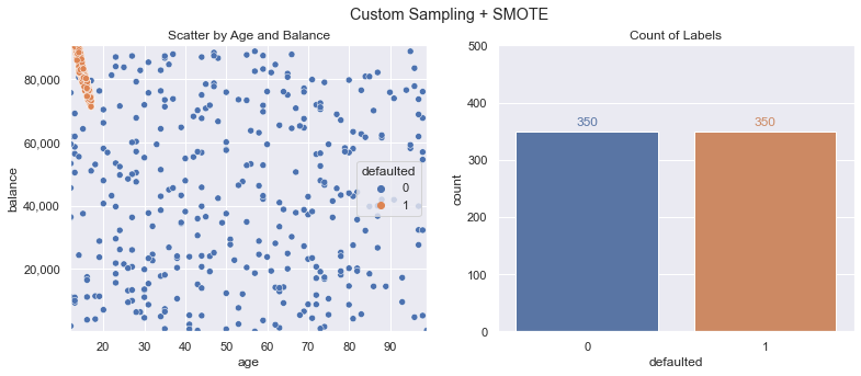
Performing SMOTE (using the same code as in the earlier steps) results in the following training dataset - creating 350 defaulted class samples from our original 10:

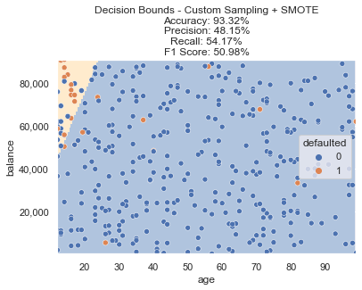
We train another new logistic regression model and using this resampled data, we now meet our goals! We can see the decision boundary now accounts for that pocket of defaults after training on our adjusted data. Accuracy is still 90%+ and F1 Score is above our goal of 50%.

Summary

There are a variety of methods to deal with imbalanced classes when building a machine learning model. Depending on your constraints, goals, and data - some may be more applicable than others. We can also come up with some creative methods for resampling in order to build a classifier that properly targets the decision bounds and scenarios we are interested in - filtering out what may appear to be noise in our data.

All examples and files available on Github.