
Exploring time series autocorrelations and change points can help familiarize with potential breakdowns in approaches. In this article, I review testing for stationarity, seasonal decomposition, autocorrelation, and change point detection.
Data Overview
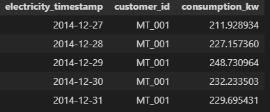
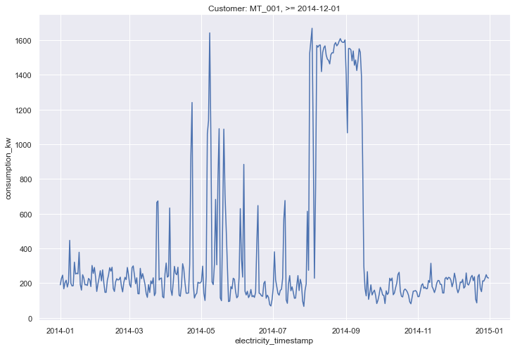
To demonstrate time series eda, we’ll use the UCI Electricity Consumption Dataset. This dataset contains electricity usage over time for various customers. The source data is rolled up to the day grain for one sample customer. The input data looks as follows:
Stationary Time Series
Some machine learning methods, such as ARIMA, rely on a stationary time series as inputs. There shouldn’t be a time-dependent structure, such as seasonality, which may cause issue with the assumptions of the forecast model.
This can be statistically tested with the Augmented Dickey-Fuller test in statsmodels. A p value <= 0.05 would suggest the time series is stationary, while > 0.05 suggest there may be some time-dependent relationship we need to take care of before forecasting.
from statsmodels.tsa.stattools import adfuller

# Run test
adf_result = adfuller(df_ts)

# Parse test statistic and p value
print(f'ADF Test Statistic {adf_result[0]:.2f}')
print(f'P Value {adf_result[1]:.2f}')
if adf_result[1] > 0.05:
    print('Time series is not stationary. Time-dependent structure such as seasonality exists.')
else:
    print('Time series is stationary, p value < 0.05.')
Output:
ADF Test Statistic -3.91
P Value 0.00
Time series is stationary p value < 0.05.Seasonal decomposition
This particular dataset doesn’t exhibit much seasonality and is showing as stationary. However, if there is seasonality to adjust for, the seasonal decomposition in statsmodels is a good place to start. Check out my previous article on seasonal decomposition for more information.
Autocorrelation
Many time series models use past values (lags) as features to forecast future values. One way of viewing this relationship in the data is through the use of autocorrelation plots. These plots show visually the correlation between the current values and past lags. Additionally, partial autocorrelation removes indirect correlations between the lags.
We can see in the charts below, the prior day value has the highest correlation.
# Autocorrelation
from statsmodels.graphics.tsaplots import plot_acf

plot_acf(df_ts)
plt.show()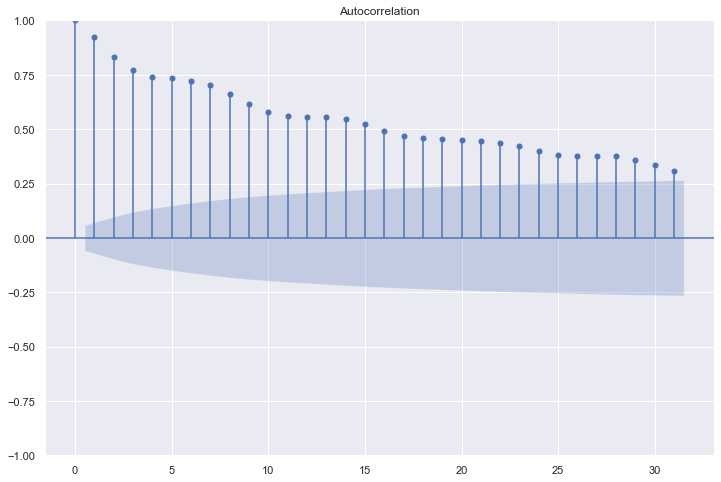
# Partial Autocorrelation
from statsmodels.graphics.tsaplots import plot_pacf

plot_pacf(df_ts, method='ywm')
plt.show()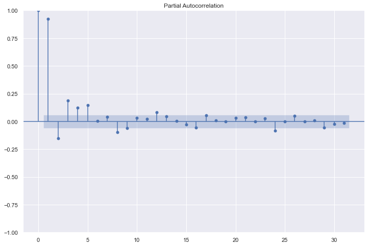
Change Point Detection
Detecting structural change points can be important to understand when major breaks in your time series occur. There could be an external variable that causes disruption in an otherwise consistent trend. Spotting these change points could lead to modeling decisions on to best handle different regimes in a longer spanning forecast.
The ruptures package is a good place to start to analyze potential change points. The below code performs a good job at identifying the major change points in this time series. Alternating colors show the different regimes and change points throughout the data.
# Model Inputs
points = np.array(df.consumption_kw)

# Define and fit model (window with 90 width and l2 loss)
algo = rpt.Window(width=90, model="l2").fit(points)

# Predict breakpoints - either manually or via penalization factor (this example)
breakpoints = algo.predict(pen=np.log(len(points)) * 2 * np.var(points)/2) # just an example, see docs for more information.

# Defining number of break points manually is also possible
# breakpoints = algo.predict(n_bkps=10) # or define number of break points manually

# Display results
rpt.show.display(points, breakpoints, figsize=(10, 6))
plt.title('Change Point Detection: Window-Based Search With Penalty Factor')
plt.show()
Summary
This is certainly only a basic overview of potential time series data exploration methods. Stationarity, seasonality, autocorrelations, and structural change points can provide a deeper understanding into what is going on within a time series - beyond just visual examination.
All examples and files available on Github.