Predicting Wine Prices with Hyperparameter Tuning

Overview

What is Hyperparameter Tuning?

Many popular machine learning libraries use the concept of hyperparameters. These can be though of as configuration settings or controls for your machine learning model. While many parameters are learned or solved for during the fitting of your model (think regression coefficients), some inputs require a data scientist to specify values up front. These are the hyperparameters which are then used to build and train the model.

One example in gradient boosted decision trees is the depth of a decision tree. Higher values yield potentially more complex trees that can pick up on certain relationships, while smaller trees may be able to generalize better and avoid overfitting to our outcome - potentially leading to issues when predicting unseen data. This is just one example of a hyperparameter - many models have a number of these inputs which all must be defined by a data scientist or alternatively use defaults provided by the code library.

This can seem overwhelming - how do we know which combination of hyperparameters will result in the most accurate model? Tuning (finding the best combination) by hand can take a long time and cover a small sample space. One approach which will be covered here is using Optuna to automate some of this work. Rather than manually testing combinations, ranges for hyperparameters can be specified and Optuna runs a study to determine the optimal combination given time constraints.

Dataset Overview

To demonstrate Optuna and hyperparameter tuning, we’ll be using a dataset containing wine ratings and prices from Kaggle. Given some input features for a bottle of red wine - such as region, points, and variety - how close can we predict the price of a wine using hyperparameter tuning?

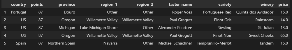
A few lines of code to load in our data and train/test split:

# Read in data from local csv
df = pd.read_csv('winemag-data-130k-v2.csv')

# Choose just a few features for demonstration, infer categorical features
feature_cols = ['country', 'points', 'province', 'region_1', 'region_2', 'taster_name', 'variety', 'winery']
cat_features = [col for col in feature_cols if df[col].dtype == 'object']
for col in cat_features:
    df[col] = df[col].fillna('Other')
target_col = 'price'

# Train test split
train_df, test_df = train_test_split(df, test_size=0.3, shuffle=False)

train_x = train_df.loc[:, feature_cols]
train_y = train_df.loc[:, target_col]

test_x = test_df.loc[:, feature_cols]
test_y = test_df.loc[:, target_col]

Model Training

Baseline Models

To know if our hyperparameter optimization is helpful, we’ll train a couple baseline models. The first is taking a simple mean price. Using this methodology results in a mean absolute percentage error of 79% - not very good, hopefully some machine learning modeling can improve our predictions!

The second baseline is training our model (using the Catboost library) with default parameters. Below are a few lines of this code. This beats our baseline simple mean prediction, but can we do better with further optimization?

# Train a model with default parameters and score
model = CatBoostRegressor(loss_function = 'RMSE', eval_metric='RMSE', verbose=False, cat_features=cat_features, random_state=42)
default_train_score = np.mean(eda.cross_validate_custom(train_x, train_y, model, mean_absolute_percentage_error))
print('Training with default parameters results in a training score of {:.3f}.'.format(default_train_score))

Output: Training with default parameters results in a training score of 0.298.

Hyperparameter Optimized Model

Setting up the optimization study

To create our model with optimized hyperparameters, we create what Optuna calls a study - this allows us to define a trial with hyperparameter ranges and optimize for the best combination.

You’ll see in the below code, we define an objective function with a trial object that suggests hyperparameters according to our defined ranges. We then create the study and optimize to let Optuna do its thing.

def objective(trial):

    # Define parameter dictionary used to build catboost model
    params = {
        'loss_function': 'RMSE',
        'eval_metric': 'RMSE',
        'verbose': False,
        'cat_features': cat_features,
        'random_state': 42,
        'learning_rate': trial.suggest_float('learning_rate', 0.001, 0.2),
        'depth': trial.suggest_int('depth', 2, 12),
        'n_estimators': trial.suggest_int('n_estimators', 100, 1000, step=50)
    }
    
    # Build and score model
    clf = CatBoostRegressor(**params)
    score = np.mean(eda.cross_validate_custom(train_x, train_y, clf, mean_absolute_percentage_error))

    return score

# Create an optuna study (minimize cost) and run optimizer
study = optuna.create_study(direction='minimize')
study.optimize(objective, timeout=1800)

Reviewing results

Optuna stores the best results in our study object. Running the below allows us to access the best trial and review training results.

# Grab best trial from optuna study
best_trial_optuna = study.best_trial
print('Best score {:.3f}. Params {}'.format(best_trial_optuna.value, best_trial_optuna.params))

Output: Best score 0.288. Params {'learning_rate': 0.0888813729642258 'depth': 12 'n_estimators': 800}

Comparing to default parameters

Doing a quick comparison of training results to our initial run with default parameters shows good signs. You’ll see that the optimized model has a better training fit (score is percentage error in this case, so lower = better).

# Compare best trial vs. default parameters
print('Default parameters resulted in a score of {:.3f} vs. Optuna hyperparameter optimization score of {:.3f}.'.format(default_train_score, best_trial_optuna.value))

Output: Default parameters resulted in a score of 0.298 vs. Optuna hyperparameter optimization score of 0.288.

Analyzing Optimization Trends

One neat thing is the parallel coordinates plot. This lets us view trials and analyze hyperparameters for potential trends. We may want to run a new study after reviewing results if we find interesting optimizations, allowing us to search additional hyperparameter spaces.

# Visualize results to spot any hyperparameter trends
plot_parallel_coordinate(study)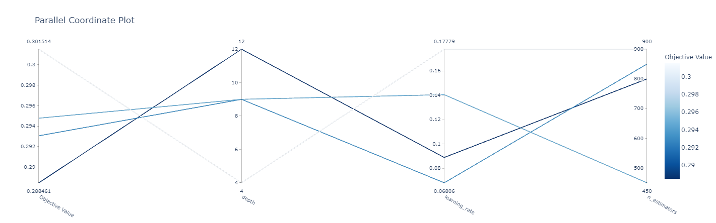

You can see the cost metric on the left (lower = better). Following the dark lines (best trials), you’ll notice a higher depth works best, a learning rate in the middle of our values tested, and a larger number of estimators. Given these findings, we could re-run a study narrowing in on these values and potentially expanding ranges of others - such as depth potentially increasing above our upper bound or adding in additional hyperparameters to tune.

Comparing Test Results

The final step is to compare test results. The first step is seeing how our simple mean prediction baseline does on the test set.

# Run baseline model (default predicting mean)
preds_baseline = np.zeros_like(test_y)
preds_baseline = np.mean(train_y) + preds_baseline
baseline_model_score = mean_absolute_percentage_error(test_y, preds_baseline)
print('Baseline score (mean) is {:.2f}.'.format(baseline_model_score))

Output: Baseline score (mean) is 0.79.

The next step is to view test results on our default hyperparameter model:

# Rerun default model on full training set and score on test set
simple_model = model.fit(train_x, train_y)
simple_model_score = mean_absolute_percentage_error(test_y, model.predict(test_x))
print('Default parameter model score is {:.2f}.'.format(simple_model_score))

Output: Default parameter model score is 0.30.

A lot better than simply using the mean as a prediction. Can our hyperparameter-optimized solution do any better on the test set?

# Rerun optimized model on full training set and score on test set
params = best_trial_optuna.params
params['loss_function'] = 'RMSE'
params['eval_metric'] ='RMSE'
params['verbose'] = False
params['cat_features'] = cat_features
params['random_state'] = 42
opt_model = CatBoostRegressor(**params)
opt_model.fit(train_x, train_y)
opt_model_score = mean_absolute_percentage_error(test_y, opt_model.predict(test_x))
print('Optimized model score is {:.2f}.'.format(opt_model_score))

Output: Optimized model score is 0.29.

Summary

We were able to improve on our model with hyperparameter optimization! We only searched a small space for a few trials, but improved our cost metric, leading to a better score (lower error by 1%).

All examples and files available on Github.